ezplot()函數與fplot()函數一樣,不需要繪圖數據陣列,只要設定一個描述函數的字串,就可運用ezplot()函數繪出指定的函數圖形。ezplot()函數使用上比fplot()函數更為簡單。
¡ezplot()函數的命令格式如下:
ezplot('fun', [xmin xmax ymin ymax], fig)
其中fun為函數的字串;[xmin xmax ymin ymax]為顯示繪圖範圍向量,其中範圍向量可以省略,其預設值為-2*pi~2*pi之間的範圍;fig為指定繪圖視窗編號。但是ezplot()函數不支援繪圖控制碼。
ezplot()函數雖與fplot()函數相似,不過卻多了繪製隱函數(implicit function)及參數式(parametric equations)圖形。
例如繪製隱函數 f(x,y) = x^4-3y^2
>> ezplot('x^4-3*y^2')
會發現自動多出圖形標題及 x 軸與 y 軸的說明。
例如繪製參數式 x = 2cos(t)-cos(30t)、y = 2sin(t)-sin(30t)圖形,t介於0~2pi之間
>> ezplot('2*cos(t)-cos(30*t)', '2*sin(t)-sin(30*t)', [0 pi 0 pi]), hold on
>> ezplot('2*cos(t)-cos(30*t)', '2*sin(t)-sin(30*t)', [pi 2*pi pi 2*pi]), hold off
註:以ezplot()函數繪製圖形時,所設定的繪圖點數有限,當圖形變化劇烈時會出現不平滑的現象,因此本例採用兩次繪圖。
或是使用內聯函數繪製參數式 x = tcos2t, y = tsin2t圖形,t介於0~4*pi之間
>> x = inline('t*cos(2*t)')
>> y = inline('t*sin(2*t)')
>> ezplot(x,y,[0 pi]*4)
fplot()函數不需要繪圖數據陣列,只要設定一個描述函數的字串,就可運用fplot()函數繪出指定的函數圖形。
¡fplot()函數的命令格式如下:
fplot('fun', [xmin xmax ymin ymax])
其中fun為函數的字串;[xmin xmax ymin ymax]為顯示繪圖範圍向量,其中xmin與xmax分別表示x軸的最小值與最大值,並且不可以省略,而ymin與ymax分別表示y軸的最小值與最大值,若省略則會依實際大小由MATLAB自動調整顯示的y軸範圍。fplot()函數也可加入線條規範語法(Line specification syntax)來指定繪圖曲線的樣式。
例如:
>> fplot('sin(x)', [-pi pi], '--ro')
>> title('sin({\itx})'), xlabel('\itx')
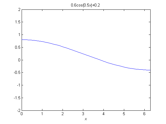
例如:
>> fplot('0.6*cos(0.5*x)+0.2', [0 2*pi -2 2])
>> title('0.6cos(0.5{\itx})+0.2'), xlabel('\itx')
此外,MATLAB提供一種簡單建立函數字串的方法-匿名函數(Anonymous function),建立方法如下:
fun = @(arg_list) expr
其中arg_list為函數的輸入引數(自變數)字串,expr為函數本體,fun為
函數名稱,使用的方式如下:
>> fun = @(x) 0.6*cos(0.5*x) + 0.2;
>> fplot(fun, [0, 2*pi, -1.5, 1.5])
>> title('0.6cos(0.5{\itx})+0.2'), xlabel('\itx')
除了使用匿名函數之外,函數字串也可以使用.m檔的函式。
例如一個fun.m檔,其內容為
function y = fun(x)
y = 0.6*cos(0.5*x) + 0.2;
在命令視窗內鍵入
>> fplot('fun', [0, 2*pi, -1.5, 1.5])
>> title('0.6cos(0.5{\itx})+0.2'), xlabel('\itx')
其結果與上圖相同 。
還有一個簡單的方法是使用內聯函數(inline function),而不需另外建立一個.m檔的函式。內聯函數是MATLAB提供的物件(object),它與函式檔性質相同,但比較容易建立。
例如:
>> fun=inline('0.6*cos(0.5*x) + 0.2');
>> fplot('fun', [0, 2*pi, -1.5, 1.5])
>> title('0.6cos(0.5{\itx})+0.2'), xlabel('\itx')
其結果也與上圖相同 。
若fplot()函數的命令格式如下:
fplot('fun', [xmin xmax ymin ymax], tol)
且tol<1,則是設定繪圖的相對容許誤差值(relative error tolerance),內定為2×10^(-3)。適度的調整tol可得到較佳的繪圖效果。
例如:
>> fun = @(x) sin(15*(3*x^3+2*x^2))./(x+1);
>> fplot(fun,[0 2])
若改為
>> fplot(fun,[0 2], 10^-5)
可發現與之前的繪圖有明顯差異。fplot()函數的另一項特點是會依據函數字串的曲線陡峭程度自動調整數據的點數,以繪出較為平滑的曲線。
此外,若fplot()函數的命令格式如下:
fplot('fun', [xmin xmax ymin ymax], N)
且N>=1,則是設定繪圖的點數最小為N+1個點,N內定為1;繪圖點的最大間距限制為(xmax-xmin)/N。
fplot()也可以指定變數來接收繪圖數據,格式如下:
[x y] = fplot('fun', [xmin xmax ymin ymax])
其中x為x軸繪圖數據,y為y軸繪圖數據。
一、繪圖函數plot
plot()函數命令格式如下:
格式一:
plot(y)
其中 y 為一向量變數。繪製圖形時,若 y 屬於為實數向量,x 軸將以 1、2、...、length(y),方式指定 x 軸座標,並以藍色" . 點"符號(預設)分別在(1,y(1))、(2,y(2))、...、(length(y),y(end))座標上顯示,再以實線(預設)依序將各座標連接起來。若 y 屬於為複數向量,x 軸將以real(y(1))、real(y(2))、...、real(y(end)),方式指定 x 軸座標(也就是y的實部),y 軸則為imag(y(1))、imag(y(2))、...、imag(y(end))(也就是y的虛部)。其中real()為取實部函數、imag()為取虛部函數、length()可回傳向量的最大列(行)數,而end指的是向量最後一個元素。
例如:
>> y=[3 2 5 7 1];
>> plot(y) % 預設為藍色.符號與實線連接
>> y=[3+3i 2-6i 5+i 7 1+5i];
>> plot(y) % 預設為藍色.符號與實線連接
格式二:
plot(x, y, LineSpec)
其中 x、y 皆為向量變數且 x、y 的元素個數須相同。繪製圖形時,若 x、y 皆屬於為實數向量,x 軸將以 x(1)、x(2)、...、x(end) 方式指定x軸座標,並以 y(1)、y(2)、...、y(end) 方式指定 x 軸座標,再以線條規範語法(Line specification syntax,LineSpec)來指定繪圖曲線的樣式。若 x 或 y 屬於為複數向量,將忽略向量虛部部份,僅以實數部份呈現繪圖座標,並提出警告訊息(Warning: Imaginary parts of complex X and/or Y arguments ignored)。
例如:
>> x=[2 4 6 7 9];
>> y=[3 2 5 7 1];
>> plot(x, y) % 預設為藍色.符號與實線連接
例如:
>> x=[2 4 6 7 9];
>> y=[3+3i 2-6i 5+i 7 1+5i];
>> plot(x, y) % 預設為藍色.符號與實線連接
Warning: Imaginary parts of complex X and/or Y arguments ignored
格式三:
plot(x1, y1, LineSpec1, x1, y1, LineSpec2, ...)
其中 x1、y1、x2、y2、...皆為向量變數。此時將可繪出多條曲線,分別為 x1、y1 ,x2、y2 曲線、...。各曲線皆依各線條規範語法LineSpec1、LineSpec1、...指定繪圖曲線的樣式。
例如:
>> x=linspace(0,2*pi,50);
>> plot(x,sin(x),'-ro',x,cos(x),':gx')
線條規範語法(Line specification syntax,LineSpec)
線條規範語法如下表所示,使用時以字串串接方式輸入,各符號的順序可以不計。
其中黃底為預設值
格式四:
plot(x, y, LineSpec, 'property1', p1, 'property2', p2 ...)
其中 x、y 皆為向量變數。此時僅能繪出一條曲線。曲線依線條規範語法LineSpec指定繪圖曲線的樣式。而各標記與線條的屬性 property1、property2、...由p1、p2、...指定。屬性的英文字母大小寫不拘。
各屬性如下:
例如:
>> x=linspace(0,2*pi,50);
>> plot(x,sin(x),'-rs','LineWidth',4,'markeredgecolor','b','markerfacecolor','m')
有時也可以使用set()函數重新定義標記與線條的屬性。
例如:
>> x=linspace(0,2*pi,50);
>> h = plot(x,cos(x),'-md'); % h為曲線的handle
接著輸入
>> set(h, 'LineWidth',2,'Markerfacecolor','b') % 指定調整曲線handle h的屬性
 繪多條曲線也可以善加運用 hold 命令。
三、
除了繪圖函數plot之外,MATLAB亦提供許多二維(2D)類型的繪圖函數。包括:
1. 簡單易使用的fplot()與ezplot()
2.對數semilogx()、semilogy()、loglog()
3.累積圖形area()
4.填色函數fill()
5.火柴棒圖stem()
6.階梯圖stairs()
7.羽毛圖feather()
8.誤差條狀圖errorbar()
9.羅盤圖compass()
10.雙y軸函數plotyy()
11.繪製梯度向量場的gradient()及quiver()
12.長條圖bar()
13.橫向長條圖barh()
14.派形圖pie()
15.直方圖(histogram)hist()
16.極座標統計圖rose()
17.彗星圖comet()---俱動態畫的繪製圖形
18.等高線圖contour()、contourc()、contourf()
19.極座標曲線圖polar()
使用 lookfor plot 可查出大部份的繪圖函數
Array環境
‘l’(flush left左齊)
’c’(centered置中)
’r’(flush right右齊)
行與行元素的間隔符號以’&’表示
列與列元素的間隔符號以’\\’表示(換行)
\left( 表示左邊的小括號,還可以是 [、{、|
\right) 表示右邊的小括號,還可以是 ]、}、|
\begin{array} 宣告一個array的數學環境
\end{array} 結束array的數學環境
{ccc} 表示3個行元素都置中(centered)
Example 5:
>>close all
>>mytexstr = '$\left(\begin{array}{ccc}a
& 14 & c\\d-3 & e & f';
>>mytexstr = [mytexstr
'\\g & h &
\lambda \end{array}\right)$'];
>>h = text('string',mytexstr,'interpreter','latex',...
'fontsize',40,'units','norm','pos',[.1 .5]);
Example 6:
>>close all
>>mytexstr = '$\left[\begin{array}{ccc}a & 14 & c\\d-3 & e & f';
>>mytexstr = [mytexstr '\\g & h & \lambda \end{array}\right]$'];
>>h = text('string',mytexstr,'interpreter','latex',...
'fontsize',40,'units','norm','pos',[.1 .5]);
\det 數學環境的det,若無’\’,則是以斜體來呈現
Example 7:
>>close all
>>mytexstr = '$\det\left|\begin{array}{lllll}a_1 & a_2 & a_3 & ';
>>mytexstr = [mytexstr '\cdots & a_n\\b_1 & b_2 & b_3 & \cdots & b_n\\ '];
>>mytexstr = [mytexstr '\vdots & \vdots & \vdots & \ddots & \vdots\\ '];
>>mytexstr = [mytexstr 'z_1 & z_2 & z_3 & \cdots & z_n \end{array}\right|>0$'];
>>h = text('string',mytexstr,'interpreter','latex',...
'fontsize',20,'units','norm','pos',[0.2 .5]);
上、下特殊效果
\stackrel{}{} 符號疊合使用\hat 重音符號 ~
\tilde 重音符號 ^
\widehat{} 寬hat
\widetilde{} 寬tilde
\overbrace{} 頂橫式大括號\underbrace{} 底橫式大括號\overline{} 頂線\underline{} 底線\vec 向量符號
Example 4:(字串過長,可分行輸入)
>>close all
>>mytexstr = '$\overbrace{\lim_{\hat{n} \rightarrow \infty}';
>>mytexstr = [mytexstr '\bar{x_5}+\overline{ymin}}='];
>>mytexstr = [mytexstr '\underbrace{\widetilde{\widehat{\tilde{y}^2+'];
>>mytexstr = [mytexstr '\underline{5}}}}\stackrel{\vec{a}}{\rightarrow}B$'];
>>h = text('string',mytexstr,'interpreter','latex',...
'fontsize',20,'units','norm','pos',[.1 .5]);
Example 1:
>> close all
>> mytexstr =
'$\frac{1}{2}$';
>> h =
text('string',mytexstr,'interpreter','latex',...
'fontsize',40,'units','norm','pos',[.5 .5]);
Example 2:
>> close all
>> mytexstr =
'$z=\frac{y^{\frac{3}{n-3}}}{x-4}$';
>> h =
text('string',mytexstr,'interpreter','latex',...
'fontsize',40,'units','norm','pos',[.5 .5]);
Example 3:
>> close all
>> mytexstr =
'$\sqrt[m]{n^3+\sqrt{x_3}}$';
>> h =
text('string',mytexstr,'interpreter','latex',...
'fontsize',40,'units','norm','pos',[.1
.5]);
數學環境格式:
$為開始或結束的符號、 \\為換行符號
可用於text( )中的符號有
可用於xlabel、ylabel、zlabel、title及text中的箭頭符號